32. Finalize the Bayes Localization Filter

We have accomplished a lot in this lesson.

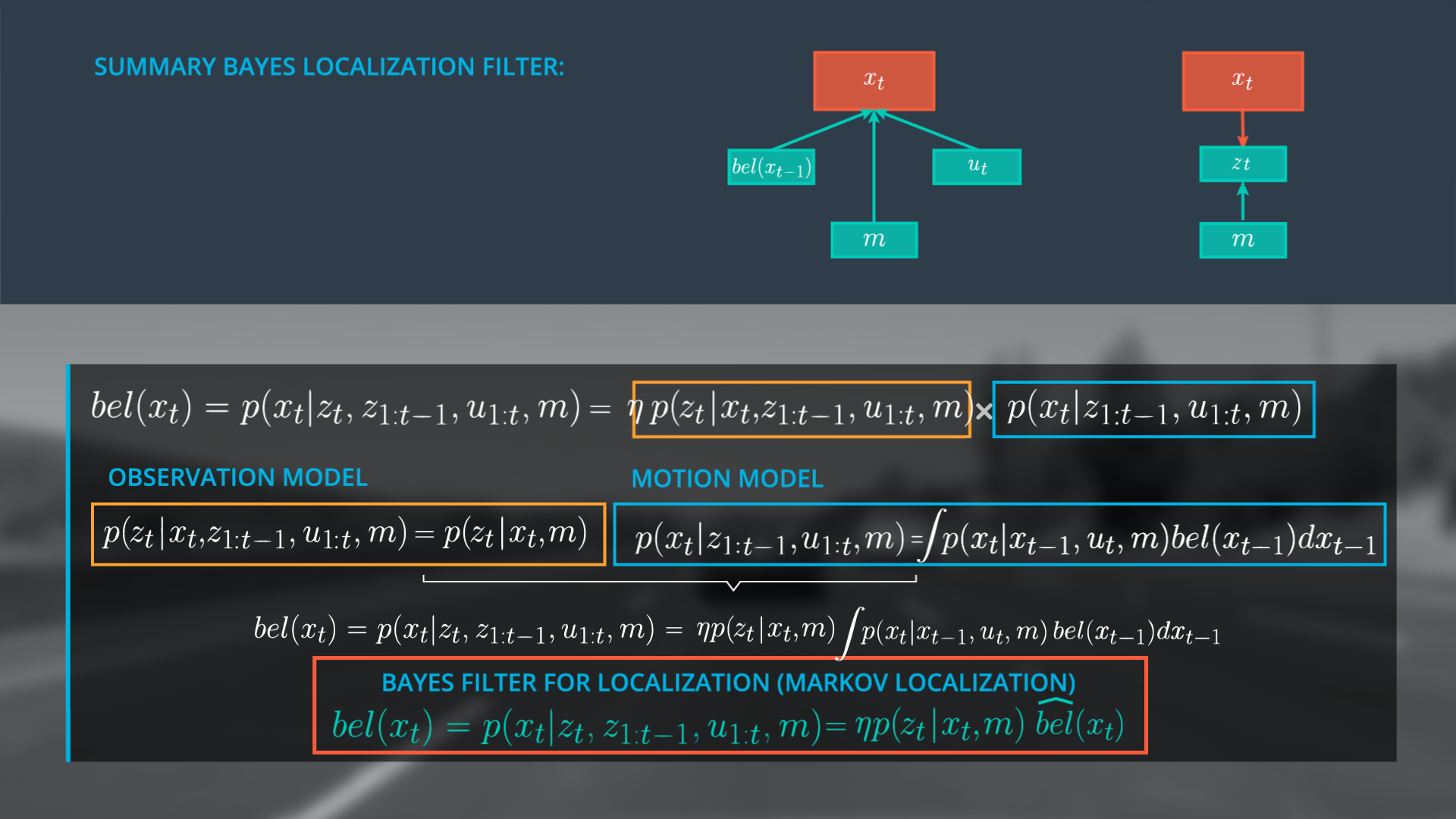
• Starting with the generalized form of Bayes Rule we expressed our posterior, the belief of x at t as \eta (normalizer) multiplied with the observation model and the motion model.
• We simplified the observation model using the Markov assumption to determine the probability of z at time t, given only x at time t, and the map.
• We expressed the motion model as a recursive state estimator using the Markov assumption and the law of total probability, resulting in a model that includes our belief at t – 1 and our transition model.
• Finally we derived the general Bayes Filter for Localization (Markov Localization) by expressing our belief of x at t as a simplified version of our original posterior expression (top equation), \eta multiplied by the simplified observation model and the motion model. Here the motion model is written as \hat{bel} , a prediction model.

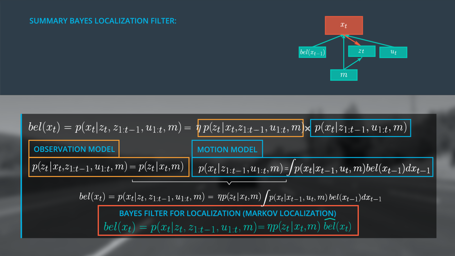
The Bayes Localization Filter dependencies can be represented as a graph, by combining our sub-graphs. To estimate the new state x at t we only need to consider the previous belief state, the current observations and controls, and the map.

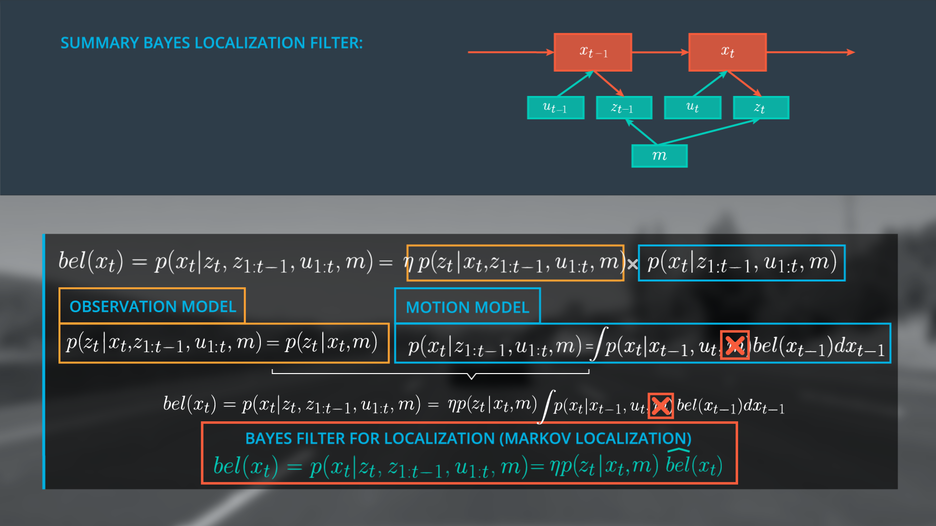
It is a common practice to represent this filter without the belief x_t and to remove the map from the motion model. Ultimately we define bel(x_t) as the following expression.

Bayes Filter for Localization (Markov Localization)